Bohr theory (English)

Top of Part 4

Last page

4-3: The Bohr Model of Atoms

The Rutherford model of the nuclear atom

had been beautifully

successful in explaining

the alpha particle scattering.

It was however

completely powerless

to explain the stability

of atoms and

to derive the atomic spectra.

As seen in the previous sections,

it brought about

a serious difficulty

which cannot be overcome

within the classical theory.

Discussing

with Rutherford in UK,

N. H. D. Bohr

(Denmark, 1885 - 1962)

learned the Rutherford model

and extended

this model to the so-called

Bohr model.

Bohr

followed Rutherford and

thought that,

in a hydrogen atom,

an electron revolves

about the proton

at such speed

that the Coulomb force

between the electron

and proton becomes

just equal to the

centrifugal force

to keep this orbital motion.

As discussed

on the preceding page,

this model

was unstable with respect

to the classical theory.

Moreover, this model

had one more difficulty.

It was known

that all hydrogen atoms

are equal to each other

and have the equal radius,

but there was nothing

in this model to assure

this equality.

Thus, if the Rutherford model

was to survive,

it was necessary to find

a radical remedy

that would bring

both the stability and the

constant radius.

To prepare the remedy,

taking a hint from

Balmer's formula

of the hydrogen spectra,

Bohr added the hypotheses

stated below to

the Rutherford model

(1913).

This model is

sometimes called

the Bohr-Rutherford model of the nuclear atom

or Bohr's quantum theory,

which was the first unified

theory to be able

to explain the

structure of the hydrogen atom

including both the stability

and the fixed radius.

[Bohr's Quantum Theory]

Bohr considered

that the electrons revolve

around the atomic nucleus

obeying the classical theory

(Newtonian mechanics

and Maxwellian electromagnetism).

He added the following

hypotheses

to the Rutherford model:

	(1)	An atom can exist only in special states with discrete (step-like) values of energy. (Electrons in an atom can exist only in certain special orbits.) Bohr called these special states (or orbits) stationary states.
	(2)	When an atom makes a transition from one stationary state to another, it emits or absorbs radiation whose frequency , is given by the frequency condition where E' and E'' are the energies of these stationary states.
	(3)	In the stationary states, the electrons move obeying the classical theory. Among the possible motions obeying the classical theory, only those satisfying the following quantum condition are realized: where p is the momentum of the electron and q is its coordinate variable. The integration should be done along the orbit over one period of the cyclic motion.

The theory constructed

on the basis of

the above hypotheses

is called

Bohr's quantum theory

or sometimes

the old quantum theory.

[The Hydrogen Atom]

Let us apply

Bohr's quantum theory

to the hydrogen atom.

Suppose that an electron

(mass = m)

revolves

around the proton

being at rest at the center

under a Coulomb attractive force.

This motion

of the electron

is described

by the Newtonian equation

of motion.

The orbit of the electron

in this case

is elliptic in general.

Now, let us assume

it to be a circle

for simplicity.

In this case the absolute value

of the momentum of

the electron, p,

is constant.

Then the quantum condition

is written

where a

is the radius of the orbit.

From the balance

of the centrifugal force

and the Coulomb force,

we have

Combining Eqs. (3) and (4),

we obtain the radius

a of the orbit as

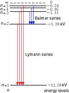
Since the energy

of the electron,

E, is the sum of

the kinetic and potential

energies, we have

Let us write this

E_n.

The allowed energies

of the hydrogen atom are

the discrete ones ,

given by

Eq. (6).

The state of n = 1

is the lowest energy state

called the ground state.

The radius of the orbit

in the ground state, a₀,

is especially called the

Bohr radius,

whose value is

This Bohr radius

is thought to be the radius

of an ordinary hydrogen atom,

and there can exist

no hydrogen atom

with a radius smaller

than this.

When the hydrogen atom

jumps (makes a transition)

from one stationary state

with the energy

E_n

to another with

E_k,

it emits or absorbs

a light whose frequency ,

is given by

the frequency condition

Eq. (1).

Using the energy

Eq. (6),

we therefore have

This is just the same as

Balmer's Formula

Rydberg's formula

which was obtained

empirically.

Therefore, the value

of the Rydberg constant

is calculated as

This result is exactly

fit to the experimental value.

Thus, Bohr's quantum theory

could beautifully reproduce

the structure of

the hydrogen atom.

[The Energy Levels and the Spectra of Hydrogen]

According to Bohr's

quantum theory,

the energy of the hydrogen atom

is given by Eq. (6).

The state of n = 1

is the ground state

which has the lowest energy.

The states of

n = 2, 3, ...

are the excited states.

These energy levels

are graphed in

the following figure

in units of eV,

where the energy E = 0

corresponds to the ionized

state of hydrogen

with the free electron at rest.

(The ionized state

means the state in which

the hydrogen nucleus,

i.e. proton,

and the electron are

completely separated.)

The Energy Levels of Hydrogen

The state of n = 1

is the ground state, and

n = 2, 3, ... are

the excited states.

The energies are

in units of eV,

being so measured

that the completely ionized state

is made to be of 0 eV.

The detailed experimental

data of the spectrum

of hydrogen are shown

in the following

figure,

where the Lymann, Balmer,

Paschen and Brackett series

are represented.

As seen in the

above figure,

these groups of spectral lines

are considered to

correspond to the

radiations emitted when

the transitions occur

from various states

to some specified state.

[The Confirmation of the Stationary States]

In Bohr's quantum theory

(or the Bohr model of atoms),

Bohr postulated that

an atom can exist only

in the stationary states

with discrete

(step-like)

values of energy.

This postulation

is quite difficult

to be understood

with the classical theory.

However, the spectrum

of the hydrogen atom

could be reproduced

beautifully.

This means that the idea

of the stationary states

appears "correct".

Therefore people

wanted to confirm

the existence of

the stationary states

directly by experiment.

This is the famous

Franck-Hertz experiment,

which was carried out by

J. Franck

(Germany, USA, 1882 - 1964)

and

G. Hertz

(Germany, 1887 - 1975).

This Hertz

is a researcher

different from

H. R. Hertz

(Germany, 1857 - 94)

who was famous

for the research

on electromagnetic waves

in the 19th century.

A schematic drawing

of the apparatus

used by Franck and Hertz

is shown in the following

Fig. (A).

Low-pressure mercury vapor

is introduced in a tube,

in which a filament F

is heated up

and electrons are

emitted from it.

The emitted electrons

are accelerated toward

the grid G

by the electric potential

between the filament F

and the grid G,

and after passing through

the grid have a

kinetic energy eV.

Then the electrons

are subjected to a small

retarding potential

before being collected

on the plate P.

If an electron loses

no energy in the course

from the filament to

the grid,

it will arrive

at the plate with the energy

and contribute to

the current measured

by the ammeter A.

However, if

is greater than

the excitation energy

of the gas atom

from the ground state

to the first excited state,

some of the electrons

will lose a part

of the kinetic energy

on colliding

with a gas atom.

Then they have insufficient

energy left to overcome the

retarding potential

Consequently, as the potential

is increased gradually,

we can find

a quick drop

of the current measured with

the ammeter A,

when the energy eV

is equal to the

excitation energy

of the gas atom.

If the potential V

is then increased again,

the current should rise,

and the second drop

would appear when eV

is equal to twice the

excitation energy.

In 1914,

Franck and Hertz

demonstrated such

energy absorption

whose experimental data

is shown in the

above Fig. (B).

As the potential V

between the filament

and the grid

is raised, the current

gradually increases,

but suddenly decreases

at V

= 4.9V.

After that, the current

increases again and

the second drop appears

at V

= 9.8V,

and the similar phenomena

are repeated.

This means that

the excitation energy

of the mercury atom

should be 4.9 eV.

It was confirmed

that this excitation energy

was just equal

to that obtained

from the spectra of mercury.

Franck and Hertz

obtained similar

experimental results

using not only mercury

but also neon, argon,

krypton and so on.

These results would be

the experimental proofs

of the Bohr's postulation of the stationary states.

Top
	Go back to the top page of Part 3. Go back to the last page. Go to the next page.